Graphs and Networks
Contents
Graphs and Networks#
Understanding complex systems often requires a bottom-up analysis. This can be done by examining the elementary parts of the system individually and then by turning the analysis towards the connection between them. A natural way of performing this type of analysis is through the use of networks or graphs.
Definition 2
A graph \(G=(V,E)\) consists of a finite set \(V\) of vertices (or nodes) and a finite set \(E\) of edges, where each edge \(e\in E\) is of the form \(e=\{u,v\}\) with \(u,v\in V\).
And we will make here the following simplifying assumptions:
we do not allow any edge to be a self-loop, i.e., an edge that starts and ends at the same vertex,
we do not allow more than one edge between any pair of vertices,
unless mentioned otherwise we will mostly consider undirected edges, that is edge \(e = \{u,v\} = \{v,u\}\).
Now, let us fix some notation and nomenclature.
Definition 3
Two vertices, \(u\) and \(v\), are called adjacent if there is an edge, \(uv\), connecting them. We can express adjacency of \(u\) and \(v\) by writing \(u\sim v.\)
Definition 4
If \(v\) is a vertex in a graph \(G\), the degree of \(v\), denoted \(\operatorname{deg}(v)\), is the number of edges adjacent to \(v\).
Definition 5
A walk in a graph is a sequence of vertices and edges \(v_0\), \(e_1\), \(v_1\), \(e_2\), \(v_2\), \(\ldots\), \(v_{k-1}\), \(e_k\), \(v_k\) such that edge \(e_i\) connects vertices \(v_{i-1}\) and \(v_i\), for \(1 \leq i \leq k\).
Definition 6
A graph \(G\) is connected if for any two vertices \(u\) and \(v\) of \(G\), there is a walk in \(G\) from \(u\) to \(v\).
The first way to store a graph into a computer is as an adjacency matrix. Given a graph \(G\) with \(n\) vertices, we start by label them from \(1\) to \(n\), then the adjacency matrix representing this graph will be an \(n\times n\) matrix whose entries are either 0 or 1, specifically
We now have much of the dictionary we need to start investigating some examples of graphs and networks that are used in applications. We will uncover some more information by working through the test cases.
A social network made of dolphins#
How can we use these abstract objects to model some systems of interest? We have said from the beginning that graphs are useful to describe pairwise interactions between vertices. We will start as usual from an example, and in particular we will focus on the network of social relationship between a population of Doubtful Sound bottlenose dolphins [Lus03]. It has been observed that gregarious, long-lived animals, such as gorillas (Gorilla gorilla), deer (Cervus elaphus), elephants (Loxodonta africanus) and bottlenose dolphins (Tursiops truncatus) rely on information transfer to exploit their habitat. Thus investigating their social structure is surely of interest.
First of all, let us fetch and load the data into the MATLAB environment
%% Loading the Network
websave('dolphins.mat','https://suitesparse-collection-website.herokuapp.com/mat/Newman/dolphins.mat');
load('dolphins.mat')
disp(Problem)
      name: 'Newman/dolphins'
     title: 'social network of dolphins, Doubtful Sound, New Zealand'
         A: [62x62 double]
        id: 2396
      date: '2003'
    author: 'D. Lusseau'
      kind: 'undirected graph'
     notes: [19x75 char]
       aux: [1x1 struct]
        ed: 'M. Newman'
The variable Problem is a struct variables containing several information,
what mostly concerns us now is the field Problem.A that contains the adjacency
matrix of our graph. We can now use MATLAB to transform it into the graph
format and visualize it
G = graph(Problem.A);
figure(1)
plot(G)
title(Problem.title)
MATLAB has experienced a low-level graphics error, and may not have drawn correctly.
Read about what you can do to prevent this issue by running this command: opengl problems,
then restart MATLAB.
To share details of this issue with MathWorks technical support, please
include this file with your service request: /home/cirdan/jogl.ex.13400

What are we seeing? In the word of the author [Lus03]:
Every time that a school of dolphins was encountered in the fjord between 1995 and 2001, each adult member of the school was photographed and identified from natural markings on the dorsal fin. This information was used to determine how often two individuals were seen together. To measure how closely two individuals were associated in the population (i.e. how often they were to be found together) I calculated a half-weight index (HWI) of association for each pair of individuals (Cairns & Schwäger 1987). This index estimates the likelihood that two individuals would be seen together compared with the likelihood of seeing any of the two individuals when encountering a school: […] Over the 7 years of observation the composition of 1292 schools was gathered. There were 64 adult individuals in this social network linked by 159 preferred companionships (edges)
Now let us try to investigate some properties of the network to infer some information on the dolphins. The first thing we want to look at are the degrees of the vertexes:
degree = G.degree;
[sorted_degree,rank] = sort(degree,'descend');
figure(2)
plot(1:G.numnodes,sorted_degree,'o');
axis([1 64 1 max(degree)])
xlabel('Vertex')
ylabel('Degree')
xticks(1:G.numnodes)
xticklabels(rank)
xtickangle(90)
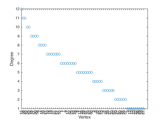
The behavior of the (reordered) degree distribution seem suspicious… let us look more into it, we call \(k\) the degree and \(p(k)\) the number of nodes with that degree
[gc,gr] = groupcounts(degree);
figure(3)
plot(gr,gc,'o')
xlabel('k')
ylabel('p(k)')
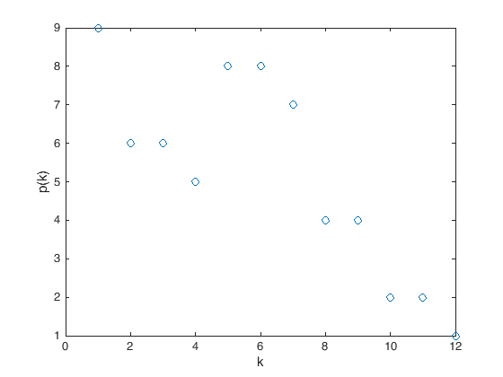
Now we observe that the behavior for smaller degree is uncertain, while the data clearly exhibit a tail (an asymptotic) that decays as a power law. Let us use the techinique for parameter estimation we have seen in the last topic for this case
fo = fitoptions('Method','NonlinearLeastSquares',...
               'Lower',[0 0],...
               'Upper',[Inf Inf],...
               'StartPoint',[1 1]);
ft = fittype('a*x.^(-b)','options',fo);
[curve,gof] = fit(gr(6:end),gc(6:end),ft);
% We plot the results
figure(1)
plot(curve,gr(6:end),gc(6:end))
xlabel('k');
ylabel('p(k)');
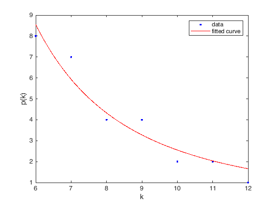
We have obtained a reasonable fit
disp(curve);
     General model:
     curve(x) = a*x.^(-b)
     Coefficients (with 95% confidence bounds):
       a =       592.1  (-381.8, 1566)
       b =       2.365  (1.523, 3.208)
with \(p(k) \sim k^{-2.365}\).
Scale-free networks
A scale-free network is a network whose degree distribution follows a power law, at least asymptotically. That is, the fraction \(p(k)\) of nodes in the network having degree \(k\) behaves for large values of \(k\) as
This type of networks have usually several properties that we can use to interpret the underlying phenomena. One of them is that they usually have a small diameter, that is, the length of the “longest shortest path”, i.e., the largest number of vertices which must be traversed in order to travel from one vertex to another when paths which backtrack, detour, or loop are excluded from consideration. We can compute it by doing
diameter = max(distances(G),[],'all');
disp(diameter)
8
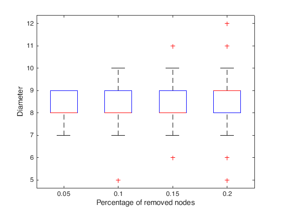
Thank to this property, dolphin scale-free network is resilient to random attacks. If we remove some random nodes the increase in the diameter is small:
percentage_of_removed = [0.05,0.10,0.15,0.20];

for j=1:length(percentage_of_removed)
    percentage = percentage_of_removed(j);
    for i = 1:500
        H = G;
        removednodes = randi(G.numnodes,floor(percentage*G.numnodes),1);
        H = H.rmnode(removednodes);
        [bin,binsize] = conncomp(H);
        idx = binsize(bin) == max(binsize);
        SG = subgraph(H, idx);
        diameters(j,i) = max(distances(SG),[],'all');
    end
end

figure(4)
boxplot(diameters.')
ylabel('Diameter')
xlabel('Percentage of removed nodes')
xticklabels(percentage_of_removed);
Finding communities#
Let us start again from an example, we consider here some data from [vDKArguellesTico+14] related to the behavior of a specie of social birds that nest in communal chambers. These contains a set of networks constructed in the following way:
An individual was assigned to a given nest chamber once it had been observed to enter it, irrespective of the activity carried out, i.e. either building the nest chamber or roosting in it. A network ‘edge’ was drawn between individuals that used the same nest chambers either for roosting or nest-building at any given time within a series of observations at the same colony in the same year, either together in the nest chamber at the same time or at different times. These individuals werethus assumed to be associated.
We read from the data file the nodes,
and edges of the network. The file (that we obtained from the Network Repository [RA15])
is not formatted as a CSV file, but has instead spaces to separate the data,
thus we use the command dlmread, that generalizes the csvread command
data = dlmread('aves-wildbird-network-1.edges');
with this we have obtained a matrix with three columns and number of edges rows in which the first column represents the starting node, the second column the ending node, and the third one the edge weight. With this data we can build a graph
G = graph(data(:,1),data(:,2),data(:,3));
and then plot it
plot(G,'Layout',"force3");
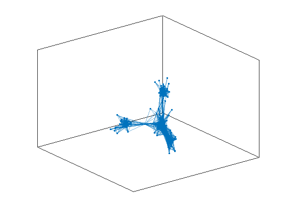
From the plot we suspect that we can identify two communities in our set of birds, but how can we do it mathematically? This task is called a task of community detection, and there are many algorithms and strategies for achieving it. We are going to focus here on a techinique that is called spectral clustering. First of all we need a particular representation of the network with a matrix called a Laplacian of the network:
L = laplacian(G);
Then we recover the spectral information by the command:
[v,l] = eigs(L,2,'smallestabs');
This gives us two vectors \(\mathbf{v}_1\) and \(\mathbf{v}_2\) and two values \(\lambda_1\) and \(\lambda_2\) such that
these are called, respectively, eigenvectors, and eigenvalues. If we inspect them we observe that \(v_1(i) > 0\) for all \(i = 1,\ldots,N\), and moreover it has a constant value. The second one, is the one we are actually interested in, this has both values that are \(> 0\) and \(< 0\). We are going to use them to determine the communities:
ind1 = find(v(:,2) > 0);
ind2 = find(v(:,2) < 0);
Now let us evidentiate the nodes on the graph
h = plot(G,'Layout',"force3");
highlight(h,ind1,"NodeColor",'red',"MarkerSize",6)
highlight(h,ind2,"NodeColor",'blue',"MarkerSize",6)
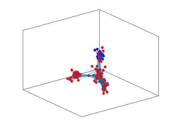
and as you can observe the procedure did evidentiate the two communities we were suspecting by working directly on the data. On the other hand, now that we look better at the data, we suspect that there could be more than two communities, the larger one seems to be splittable in two. We can try to identify larger number of communities, by computing more eigenvectors
[v,l] = eigs(L,3,'smallestabs');
idx = kmeans(v(:,2:3),3);
ind1 = find(idx == 1);
ind2 = find(idx == 2);
ind3 = find(idx == 3);
h = plot(G,'Layout',"force3");
highlight(h,ind1,"NodeColor",'red',"MarkerSize",6)
highlight(h,ind2,"NodeColor",'blue',"MarkerSize",6)
highlight(h,ind3,"NodeColor",'green',"MarkerSize",6)
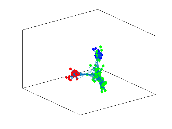
now we don’t have a clear cut between positive and negative values in a single vector, thus we have to employ another algorithm to do the separation for us. This is the \(K\)-means algorithm that returns as a vector of indexes for the corresponding communities.
Tip
\(K\)-means is a clustering method that uses the process of vector quantization, it was originally devised in the signal processing community with the aims of partitioning \(n\) observations into \(k\) clusters in which each observation belongs to the cluster with the nearest mean, i.e., the mean servs as a prototype of the cluster.
It can be formally expressed as the minimization problem
where we are given \(\{\mathbf{x}_1,\ldots,\mathbf{x}_n\}\) observations, to cluster in \(k\,(\leq n)\) groups \(\{S_1,\ldots,S_k\}\), and \(\mathbf{\mu}_i\) is the mean of the points in \(S_i\).
But how do we know if we haven’t lost some community in our analysis? To test this idea we can use another concept from graph theory that is called modularity.
Definition 7
Modularity is a measure of the structure of networks or graphs which measures the strength of division of a network into communities, it is computed as the fraction of the edges that fall within the given groups minus the expected fraction if edges were distributed at random.
There are several ways for computing this quantity, we give here a very straigthforward
function Q = modularity(A, g)
%% MODULARITY computes the modularity of the of the partition in group g of the
% graph with adjacency matrix A.

nCommunities = numel(unique(g));
nNodes = length(g);

e = zeros(nCommunities);
for i = 1:nNodes
    for j = 1:nNodes
        e(g(i), g(j)) = e(g(i), g(j)) + A(i, j);
    end
end
nEdges = sum(A(:));  % we could use nnz(A), but we want to take into account weights
a_out = sum(e, 2);   % out-degree
a_in = (sum(e, 1))'; % in-degree
a = a_in.*a_out/nEdges^2;
Q = trace(e)/nEdges - sum(a);

end
and we try to use it to evaluate the communities we have found
%% Analysis of Community Structure
addpath('matlabcodes')
data = dlmread('aves-wildbird-network-1.edges');
color = {'red','blue','magenta','green'};
G = graph(data(:,1),data(:,2),data(:,3));
L = laplacian(G);
for i = 1:3
    [v,l] = eigs(L,i+1,'smallestabs');
    groupvec = kmeans(v(:,2:i+1),i+1);
    figure(1)
    subplot(1,3,i);
    h = plot(G,'Layout',"force3");
    for j = 1:i+1
       ind = find(groupvec == j);
       highlight(h,ind,"NodeColor",color{j},"MarkerSize",6)
    end
    Q = modularity(adjacency(G),groupvec);
    title(['Modularity is ',string(Q)])
end
set(gcf,'Position',[-1984 426 1301 395]);
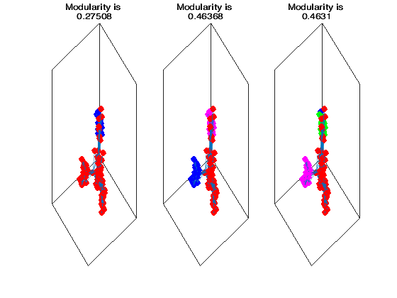
from which we observe that if we try to find more than three communities the modularity starts decreasing. Thus it seems that we are done with three communities for this dataset.
Exercise 8
We write a function that looks for in a graph up to \(n\) communities and returns the number of communities within \(n\) with the highest modularity.
function [groups,outmodularity,optimum] = findcommunities(G,k)
%%FINDCOMMUNITIES looks in G up to n communities and returns the number
%of communities within n with the highest modularity.
%   G = graph
%   k = maximum number of communities

if (k > G.numnodes)
    error("You cannot have more than number of nodes communities");
end
if (k < 2)
    error("You cannot have less than 2 communities");
end

% Allocate the space for the groups matrix of number of nodes rows and
% k-1 columns

% Allocate the space for the modularities: vector with k-1 entries

% Loop through the possible community size
% | Compute eigenvectors
% | Use k-means
% | Compute modularity
% end of the for loop

% Compute the index for which maximum modularity is obtained

end
You can test the algorithm on some of the networks on some Animal social networks.
Tip
To ensure that the function also automatically produces graphs highlighting the communities, the following two auxiliary codes can be used:
Generate maximally perceptually-distinct colors This function generates a set of colors which are distinguishable by reference to the “Lab” color space, which more closely matches human color perception than RGB.
neatly arrange subplots Sometimes a graphing function will not know in advance how many sub-plots are to be created. This function produces reasonable values for the row and column inputs to subplot given the number of desired sub-plots.
Centrality#
The next type of analysis we want to address is the computation of a node centrality score, this type of analysis can (usually) be done by employing some topological measures, i.e., that depends only on the connections of the nodes, to score nodes by their “importance”.
Definition 8
A graph Centrality measures are scalar values given to each node in the graph \(G = (V,E)\) to quantify its importance. The definition of what is important depends on the underlying model assumption.
Let us see some measures on a sample graph \(G = (V,E)\) that could be, e.g., the contact network ia-infect-hyper.mtx where nodes represent humans and edges between them represent proximity, i.e., a contact for a given period of time in the physical world; see [RA15].
addpath('./data')
data = dlmread('ia-infect-hyper.mtx',' ',2,0);
G = graph(data(:,1),data(:,2));
fprintf("G is a Network with %d nodes and %d edges.\n",G.numnodes,G.numedges);
G is a Network with 113 nodes and 2196 edges.
Degree centrality. It is defined as the number of node neighbors for each node in the graph. If the network is directed, we have two versions of this measure: the in-degree is the number of incoming edges, and the out-degree that is in turn the number of out-going edges. This is a local measure, that means that as a measure it doesn’t take neighbors connectivity into account. It can be interpreted as a form of popularity.
degree_centrality = G.degree;
Closeness centrality. This centrality measures node efficiency in terms of connection to other nodes. Is defined as the average length of the shortest path between the node and all other nodes in the graph, i.e., the more central a node is, the closer it is to all other nodes.
closeness_centrality = centrality(G,"closeness");
Betweenness centrality. This measure quantifies the number of times a node acts as a bridge along the shortest path between two other nodes, that is, let us say that we want to compute it for a vertex \(v \in V\). We first compute all the shortest paths between each pair of vertices \((s,t)\), then for each of the couples we determine the fraction of shortest paths that pass through \(v\). The measure is then the sum this fraction over all pairs of vertices, succinctly
betweenness_centrality = centrality(G,"betweenness");
Eigenvector centrality. It assigns relative scores to all nodes in the network based on the assumption that “connections to important nodes matters more to the score of the node we are looking at than equal connections to low importance nodes”. This idea can be formalized in different ways. The first we consider is the case in which we use the eigenvector corresponding to the largest eigenvalue of the graph adjacency matrix.
eigenvector_centrality = centrality(G,"eigenvector");
PageRank. This is the algorithm used by Google Search to rank the web pages in their search engine results. The score given by this algorithm is a probability distribution representing the likelihood of randomly exploring the network and arriving at any particular page.
pagerank_centrality = centrality(G,"pagerank");
We can now try to look at the most-important nodes for the different measures.
Since we are only interested in the ranking (and not in the actual value of
the measure) we will make use of the sort function from MATLAB to get the
information we want
[~,degree_rank] = sort(degree_centrality,"descend");
[~,closeness_rank] = sort(closeness_centrality,"descend");
[~,betweenness_rank] = sort(betweenness_centrality,"descend");
[~,eigenvector_rank] = sort(eigenvector_centrality,"descend");
[~,pagerank_rank] = sort(pagerank_centrality,"descend");

rankings = table(degree_rank,closeness_rank,betweenness_rank,...
    eigenvector_rank,pagerank_rank,'VariableNames',...
    {'Degree','Closeness','Betweenness','Eigenvector','PageRank'});
disp(head(rankings))
Degree Closeness Betweenness Eigenvector PageRank
______ _________ ___________ ___________ ________
30 30 30 30 30
38 38 42 102 42
42 42 33 38 38
102 102 38 42 102
33 33 102 33 33
48 48 12 48 48
12 12 48 34 12
34 34 34 12 34
To compare the different rankings we can also look at the scatter plot of the rankings, e.g.,
figure(1)
subplot(1,2,1);
plot(degree_rank,closeness_rank,'o');
xlabel('Degree centrality')
ylabel('Closeness centrality')
axis square
subplot(1,2,2);
plot(degree_rank,eigenvector_rank,'o');
xlabel('Degree centrality')
ylabel('Eigenvector centrality')
axis square
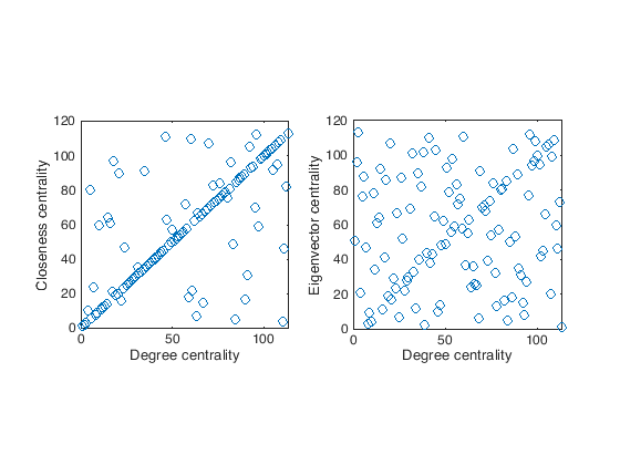
In general it would be better to have also a quantitative way of comparing the rankings. We can go for a statistical test, in this case a good solution is the Kendall \(\tau\) test.
The Kendall \(\tau\) coefficient is defined as:
Where \({n \choose 2} = {n (n-1) \over 2}\) is the binomial coefficient for the number of ways to choose two items from \(n\) items. We can compute it in MATLAB (together with the relevant \(p\)-value) by doing:
[tau,pval] = corr(degree_rank,closeness_rank,'type','Kendall');
fprintf("Degree vs Closeness tau = %f p-value = %e.\n",tau,pval);
[tau,pval] = corr(degree_rank,eigenvector_rank,'type','Kendall');
fprintf("Degree vs Eigenvector tau = %f p-value = %e.\n",tau,pval);
Degree vs Closeness tau = 0.581226 p-value = 7.253673e-20.
Degree vs Eigenvector tau = 0.099558 p-value = 1.185833e-01.
Warning
Every centrality measure is based on an assumption about the concept of importance, e.g, closeness and betweenness centralities define the importance as an evaluation of the information exchange efficiency within the networks. Others like the degree are purely local popularity measure, while the ones based on the eigenvectors tend to reward highly connected nodes. You should always select your measure while taking into account the model behind the choice.
Bibliography#
- Lus03(1,2)
David Lusseau. The emergent properties of a dolphin social network. Proceedings of the Royal Society of London. Series B: Biological Sciences, 270(suppl_2):S186–S188, 2003.
- RA15(1,2)
Ryan A. Rossi and Nesreen K. Ahmed. The network data repository with interactive graph analytics and visualization. In AAAI. 2015. URL: https://networkrepository.com.
- vDKArguellesTico+14
Rene E van Dijk, Jennifer C Kaden, Araceli Argüelles-Ticó, Deborah A Dawson, Terry Burke, and Ben J Hatchwell. Cooperative investment in public goods is kin directed in communal nests of social birds. Ecology letters, 17(9):1141–1148, 2014.