Working with images
Up to now we have worked with numerical data (data from experiments to be adapted to models, simulations of differential equations) and relational data (networks). This isn’t the only type of data you can happen to be dealing with. Another rather frequent occurrence is that of having to analyze images from various sources. We will deal here with the solution of some problems that concern them.
The first issue we have to solve, is indeed interfacing the computer with this type of data. MATLAB commands can read, write, and display several types of image file formats:
BMP
GIF
HDF
JPEG
PCX
PNG
TIFF
XWD
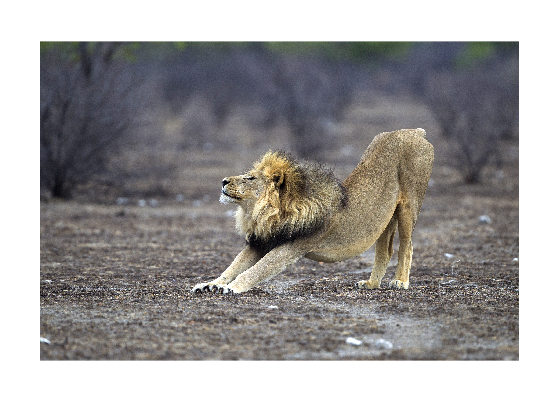
Let us start by downloading from the internet a cat photo and loading it into MATLAB:
websave('cat.jpg','https://upload.wikimedia.org/wikipedia/commons/5/52/Panthera_leo_stretching_%28Etosha%2C_2012%29.jpg');
A = imread("cat.jpg");
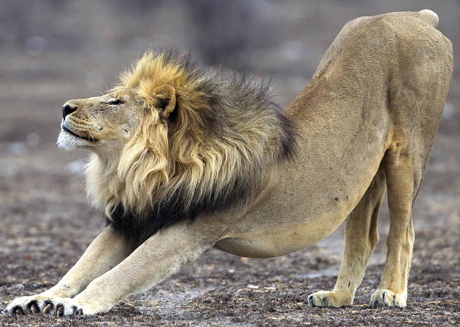
As we have seen many times, the fundamental data in MATLAB is the array, and
thus the variable A we have obtained with the imread command is indeed a
type of array. In many cases, images can be represented by using matrices, in
which entry corresponds to a single pixel of the given image. Some images,
for example RGB color images, require instead a tensor to be represented, that
is, if you prefer, a three-dimensional array. In the first plane (with respect
to the third dimension) we represent the red pixel intensities, in the second
one we represent the green pixel intensities, and finally in the third one
the blue pixel intensities.
Indeed, if we query for the variable we have just created, we find as much
whos A
  Name         Size                   Bytes  Class    Attributes

  A         2000x3000x3            18000000  uint8
that is \(A\) is a vector of integers of sizes \(2000 \times 3000 \times 3\). We can look at the figure it represents by doing
imshow(A);
Other general utility functions that we can consider are
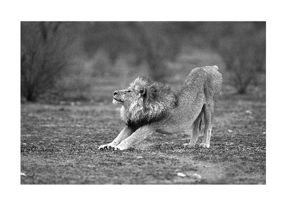
converting an RGB image to grayscale
Agray = rgb2gray(A);
imshow(Agray);
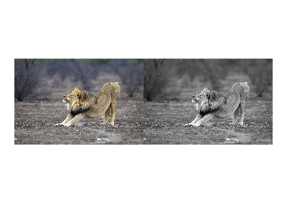
create a tiled image from multiple images
tile = imtile({A,Agray});
imshow(tile);
cropping and saving a reduced size image
image(A); axis image;
p = ginput(2);
% Get the x and y corner coordinates as integers
sp(1) = min(floor(p(1)), floor(p(2))); %xmin
sp(2) = min(floor(p(3)), floor(p(4))); %ymin
sp(3) = max(ceil(p(1)), ceil(p(2)));   %xmax
sp(4) = max(ceil(p(3)), ceil(p(4)));   %ymax
CroppedA = A(sp(2):sp(4), sp(1): sp(3),:);
figure; image(CroppedA); axis image
imwrite(CroppedA,'cropped_cat.jpg');
in which we have used the ginput command to get the coordinates of some
points from the figure, and the imwrite command to save the cropped figure
to a file.
obtaining information about graphics files (maybe useful before loading them)
iminfo = imfinfo('cat.jpg')
Warning: Division by zero when processing .  The value has been set to NaN.
> In matlab.io.internal.imagesci.imjpginfo>incorporate_exif_metadata (line 68)
In matlab.io.internal.imagesci.imjpginfo (line 51)
In imjpginfo (line 20)
In imfinfo (line 234)
iminfo =

  struct with fields:

           Filename: '/home/cirdan/Documenti/RTDa-PISA/Didattica/NumRecipes/recipesforenvsciences/src/cat.jpg'
        FileModDate: '23-Mar-2022 23:20:15'
           FileSize: 5210752
             Format: 'jpg'
      FormatVersion: ''
              Width: 3000
             Height: 2000
           BitDepth: 24
          ColorType: 'truecolor'
    FormatSignature: ''
    NumberOfSamples: 3
       CodingMethod: 'Huffman'
      CodingProcess: 'Sequential'
            Comment: {}
               Make: 'Canon'
              Model: 'Canon EOS-1D Mark IV'
        Orientation: 1
        XResolution: 240
        YResolution: 240
     ResolutionUnit: 'Inch'
           Software: 'Adobe Photoshop CS2 Windows'
           DateTime: '2014:01:26 13:25:17'
             Artist: 'Yathin Krishnappa'
          Copyright: 'yathin.com'
      DigitalCamera: [1x1 struct]
      ExifThumbnail: [1x1 struct]
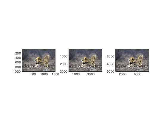
resizing images, if you want to enlarge a figure you need to guess somehow the value of the missing pixels, similarly, if you reduce it, you have to decide how to modify the remaining ones. This is done via an interpolation kernel function that calculates the value of a pixel using a weighted average of neighboring pixel values
subplot(1,3,1)
Ares = imresize(A, 0.5, "Method","bicubic");
image(Ares); axis image;
subplot(1,3,2)
Ares = imresize(A, 1.5, "Method","bilinear");
image(Ares); axis image;
subplot(1,3,3)
Ares = imresize(A, 3, "Method","nearest");
image(Ares); axis image;
Denoising images
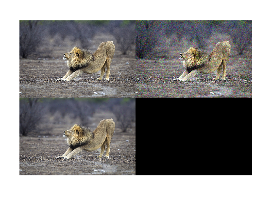
A part from photos of cats sometimes we get photos from experimental instruments that are littered with noise, and that we wish to remove. This may be either for simply having a better looking photo, or as a first step in a following analysis.
From the wavelet Toolbox you can use the following procedure to denoise an image:
Anoise = imnoise(A,'gaussian',0,0.01);
tile = imtile({A,Anoise});
imshow(tile);
Adenoise = wdenoise2(Anoise);
tile = imtile({A,Anoise,uint8(Adenoise)});
imshow(tile);
Tip
A wavelet transforms of a given signal of finite energy acts as a projection on a continuous family of frequency bands. We can represent, for instance, the signal could be represented on every frequency band \([f,2f]\) for all \(f > 0\), for example for \(f = 1\) one could select the function
and for the bands \([1/a,2/a]\) by the function
Then a signal \(x(t)\) can be decomposed as
Since it is computationally intractable to analyze a continuous signal this way, we usually reduce to a smaller set of discrete coefficients
In any case, when we have computed the coefficient, what we do to denoise the image is to throw away the “small one” that are mostly noises, while the “large ones” contain actual signal.
Further options can be analyzed by looking at the help wdenoise2.
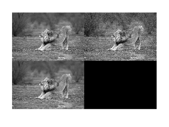
This is a classic way of solving this kind of problem. In recent times, another widely used approach is that of neural networks. The Image Processing MATLAB Toolbox has a pretrained neural network for denoising black and white images, it can be called by doing:
Agray = rgb2gray(A);
Agraynoise = imnoise(Agray,'gaussian',0,0.01);
net = denoisingNetwork('DnCNN');
Adenoisenet = denoiseImage(Agraynoise,net);
tile = imtile({Agray,Agraynoise,uint8(Adenoisenet)});
imshow(tile);
the network denoisingNetwork('DnCNN') is a rather complex object whose
structure can be investigated by doing
disp(net.Layers)
59x1 Layer array with layers:
1 'InputLayer' Image Input 50x50x1 images
2 'Conv1' Convolution 64 3x3x1 convolutions with stride [1 1] and padding [1 1 1 1]
3 'ReLU1' ReLU ReLU
4 'Conv2' Convolution 64 3x3x64 convolutions with stride [1 1] and padding [1 1 1 1]
5 'BNorm2' Batch Normalization Batch normalization with 64 channels
6 'ReLU2' ReLU ReLU
7 'Conv3' Convolution 64 3x3x64 convolutions with stride [1 1] and padding [1 1 1 1]
8 'BNorm3' Batch Normalization Batch normalization with 64 channels
9 'ReLU3' ReLU ReLU
10 'Conv4' Convolution 64 3x3x64 convolutions with stride [1 1] and padding [1 1 1 1]
11 'BNorm4' Batch Normalization Batch normalization with 64 channels
12 'ReLU4' ReLU ReLU
13 'Conv5' Convolution 64 3x3x64 convolutions with stride [1 1] and padding [1 1 1 1]
14 'BNorm5' Batch Normalization Batch normalization with 64 channels
15 'ReLU5' ReLU ReLU
16 'Conv6' Convolution 64 3x3x64 convolutions with stride [1 1] and padding [1 1 1 1]
17 'BNorm6' Batch Normalization Batch normalization with 64 channels
18 'ReLU6' ReLU ReLU
    19   'Conv7'                  Convolution           64 3x3x64 convolutions with stride [1  1] and padding [1  1  1  1]
    20   'BNorm7'                 Batch Normalization   Batch normalization with 64 channels
21 'ReLU7' ReLU ReLU
22 'Conv8' Convolution 64 3x3x64 convolutions with stride [1 1] and padding [1 1 1 1]
23 'BNorm8' Batch Normalization Batch normalization with 64 channels
24 'ReLU8' ReLU ReLU
25 'Conv9' Convolution 64 3x3x64 convolutions with stride [1 1] and padding [1 1 1 1]
26 'BNorm9' Batch Normalization Batch normalization with 64 channels
    27   'ReLU9'                  ReLU                  ReLU
    28   'Conv10'                 Convolution           64 3x3x64 convolutions with stride [1  1] and padding [1  1  1  1]
29 'BNorm10' Batch Normalization Batch normalization with 64 channels
30 'ReLU10' ReLU ReLU
31 'Conv11' Convolution 64 3x3x64 convolutions with stride [1 1] and padding [1 1 1 1]
32 'BNorm11' Batch Normalization Batch normalization with 64 channels
33 'ReLU11' ReLU ReLU
34 'Conv12' Convolution 64 3x3x64 convolutions with stride [1 1] and padding [1 1 1 1]
35 'BNorm12' Batch Normalization Batch normalization with 64 channels
36 'ReLU12' ReLU ReLU
37 'Conv13' Convolution 64 3x3x64 convolutions with stride [1 1] and padding [1 1 1 1]
38 'BNorm13' Batch Normalization Batch normalization with 64 channels
    39   'ReLU13'                 ReLU                  ReLU
    40   'Conv14'                 Convolution           64 3x3x64 convolutions with stride [1  1] and padding [1  1  1  1]
41 'BNorm14' Batch Normalization Batch normalization with 64 channels
42 'ReLU14' ReLU ReLU
    43   'Conv15'                 Convolution           64 3x3x64 convolutions with stride [1  1] and padding [1  1  1  1]
    44   'BNorm15'                Batch Normalization   Batch normalization with 64 channels
45 'ReLU15' ReLU ReLU
46 'Conv16' Convolution 64 3x3x64 convolutions with stride [1 1] and padding [1 1 1 1]
47 'BNorm16' Batch Normalization Batch normalization with 64 channels
    48   'ReLU16'                 ReLU                  ReLU
    49   'Conv17'                 Convolution           64 3x3x64 convolutions with stride [1  1] and padding [1  1  1  1]
50 'BNorm17' Batch Normalization Batch normalization with 64 channels
51 'ReLU17' ReLU ReLU
52 'Conv18' Convolution 64 3x3x64 convolutions with stride [1 1] and padding [1 1 1 1]
53 'BNorm18' Batch Normalization Batch normalization with 64 channels
54 'ReLU18' ReLU ReLU
55 'Conv19' Convolution 64 3x3x64 convolutions with stride [1 1] and padding [1 1 1 1]
56 'BNorm19' Batch Normalization Batch normalization with 64 channels
57 'ReLU19' ReLU ReLU
58 'Conv20' Convolution 1 3x3x64 convolutions with stride [1 1] and padding [1 1 1 1]
59 'FinalRegressionLayer' Regression Output mean-squared-error with response 'Response'
We could train a new network for this task, but this is a rater complex topic, and a computationally intensive task. Therefore, we are not going to pursue it.
Deblurring images
The blurring of an image can be caused by many factors, the classical are
a movement during the image capture process, e.g., a slight movement of the camera or even a micro-movement if long exposure times are used,
an out-of-focus optics,
the use of a wide-angle lens,
an atmospheric turbulence for telescopic images,
a too a short exposure time, e.g., the phenomena is very fast,
the presence of scattered light and light distortion in confocal microscopy.
As many other things we have seen until now in this course, a blurred image can be described (at least approximately) by a linear equation:
where \(\mathbf{x}\) is the image we would like to have, \(\mathbf{y}\) is the image we got from the measurement procedure, \(\mathbf{e}\) the noise vector, and \(H\) the so-called blur operator that encodes one of the blurring phenomena.
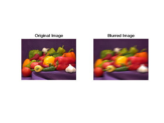
As we have done for the noise problem, we start by creating a fictitious blurred image. To reduce the computation time, we use a smaller example than the lion that is distributed with MATLAB
% First we read and visualize the image:
I = im2double(imread('peppers.png'));
figure(1)
subplot(1,2,1);
imshow(I);
title('Original Image');
% We create the operator H by using a PSF function
LEN = 31;
THETA = 11;
PSF = fspecial('motion',LEN,THETA);
Blurred = imfilter(I,PSF,'circular','conv');
figure(1);
subplot(1,2,2);
imshow(Blurred);
title('Blurred Image');
We need to discuss several aspects of these commands, first of all we need to describe how we build the \(H\) operator. This is done through the usage of a Point Spread Function (PSF), this function describes the response of the imaging system we are using when solicited by a point source. If we have in mind the model of a camera, this essentially tells us how a single ray of light (the point source) is distorted by the equipment we are using.
We produce a synthetic response by means of the fspecial function, its
help produce
fspecial Create predefined 2-D filters.
   H = fspecial(TYPE) creates a two-dimensional filter H of the
   specified type. Possible values for TYPE are:

     'average'   averaging filter
     'disk'      circular averaging filter
     'gaussian'  Gaussian lowpass filter
     'laplacian' filter approximating the 2-D Laplacian operator
     'log'       Laplacian of Gaussian filter
     'motion'    motion filter
     'prewitt'   Prewitt horizontal edge-emphasizing filter
     'sobel'     Sobel horizontal edge-emphasizing filter
that proposes several type of filters. We selected a motion blur, that
represents a linear motion of a camera by LEN pixels, with an angle of THETA
degrees in a counter-clockwise direction. Then, we build the operator \(H\) by
using the imfilter function. This operation needs the image on which we want
to apply the the filtering, the PSF, the way in which we decide to model the
boundaries of the image:
B = imfilter(A,H,OPTION1,OPTION2,...) performs multidimensional
filtering according to the specified options.  Option arguments can
have the following values:

- Boundary options

    X            Input array values outside the bounds of the array
                 are implicitly assumed to have the value X.  When no
                 boundary option is specified, imfilter uses X = 0.

    'symmetric'  Input array values outside the bounds of the array
                 are computed by mirror-reflecting the array across
                 the array border.

    'replicate'  Input array values outside the bounds of the array
                 are assumed to equal the nearest array border
                 value.

    'circular'   Input array values outside the bounds of the array
                 are computed by implicitly assuming the input array
                 is periodic.
This is a crucial part, we need to guess how the image behaves out of the
picture frame. This value are needed to close the model equation. For this test
case we selected the circular option, that assumes that the values at the
boundary are periodic. The last option decides how the PSF is transformed into
the operator \(H\)
- Correlation and convolution

    'corr'       imfilter performs multidimensional filtering using
                 correlation, which is the same way that FILTER2
                 performs filtering.  When no correlation or
                 convolution option is specified, imfilter uses
                 correlation.

    'conv'       imfilter performs multidimensional filtering using
                 convolution.
Following the intuition behind the choice of the camera model, we decide for
a conv process. At the end of this whole procedure, the variable Blurred
contains the deteriorated image that we want to restore.
To complete the problem to a realistic solution, we need to also add some noise to the image. We have seen this procedure already in the previous section.
BlurredNoised = imnoise(Blurred,'gaussian',0,0.001);
figure(2)
imshow(BlurredNoised);
title('Image to be restored');
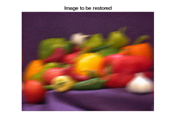
Now that we have the problem we want to solve, we can look at the routine proposed by MATLAB to solve this problem.
We use the deconvwnr function, this function requires as inputs the PSF, and
the noise-to-signal-power ratio, let us start by looking at what happens if we miss the
level of noise. As an example, let us suppose that we underestimate it, and
decide that our image has no noise whatsoever:
nsr = 0;
Restored = deconvwnr(BlurredNoised,PSF,nsr);
imshow(Restored);
With this poor choice the algorithm is incapable of finding anything useful. We end up with a worse reconstruction than the image we had start with. In principle the problem we are trying to solve is nothing more than a linear system, the problem is that we do not want to solve it completely, if we do a complete solution we end up recovering only noise! Thus, many of the algorithms for this task require that the user provide an estimate of the noise. This is used to halt the solution procedure at a point in which the obtained solution makes sense. Thus, let us try with a better guess:
nsr = 0.001 / var(I(:));
Restored = deconvwnr(BlurredNoised,PSF,nsr);
figure(3)
imshow(Restored);

That is indeed a better result.
To have a complete introduction to this type of problems a good starting point is the book [Han10], there are then a number of books covering specific aspects ranging from the atmosphere [DTS10] to geophysical [Sun13, Zhd02].
Bibliography
- DTS10
Adrian Doicu, Thomas Trautmann, and Franz Schreier. Numerical regularization for atmospheric inverse problems. Springer Science & Business Media, 2010.
- Han10
Per Christian Hansen. Discrete inverse problems. Volume 7 of Fundamentals of Algorithms. Society for Industrial and Applied Mathematics (SIAM), Philadelphia, PA, 2010. ISBN 978-0-898716-96-2. Insight and algorithms. URL: https://doi.org/10.1137/1.9780898718836, doi:10.1137/1.9780898718836.
- Sun13
Ne-Zheng Sun. Inverse problems in groundwater modeling. Volume 6. Springer Science & Business Media, 2013.
- Zhd02
Michael S Zhdanov. Geophysical inverse theory and regularization problems. Volume 36. Elsevier, 2002.