Reading, writing and plotting data
One of the transverse usages of MATLAB is as a tool for analyzing and plotting data coming from the most various sources. This material covers the commands and the ideas we may need to perform these tasks.
As you should remember from the introduction to the language, in MATLAB the most natural way of representing data is with matrices, scalars are \(1\times 1\) matrices. But how can you populate these matrices with the data coming from your experiments? Are always matrices the right format?
We will start with an example, from here you can download a csv file containing information on the quantity of pm2 particles from pollution stations in the city of London in 2019.
Tip
CSV stands for comma-separated values. These are delimited text files which use a comma to separate values. Each line of the file is a data record. Each record consists of one or more fields, separated by commas.
In most of them the separator is indeed a comma, and this justifies the source of the name for the format. Nevertheless, this is not always the case, and other delimiters can be found. In well formatted files each line will have the same number of fields.
Let us work with the data we have just downloaded. First of all, we create
a new MATLAB script called londonpollution.m, and we put the downloaded
data in the same folder of the script
%% London Pollution Data
% Analysis of the Pollution data from London.

clear; clc; close all;
If you look at the first lines of the CSV file you have downloaded, you will
see that in the same file appear different types of data, strings, numbers,
datetime, and so on. This means that we cannot store all these information
in a matrix. Matrices only take data of homogeneous type. The right type of
variable to use is a table.
We use the command readtable to load all this information into MATLAB
london = readtable('london_combined_2019_all.csv');
After these are in memory, you can get some information on the variable by writing in the command line:
whos london
and getting the answer
Name            Size               Bytes  Class    Attributes
london      24676x9             16527487  table
that tells us that we have loaded a table with 24676 rows, divided in 9 columns. Again from the command window we can look at what are the first rows by doing:
head(london)
that prints out
>> head(london)

ans =

  8×9 table

      city      latitude    longitude    country            utc                       location               parameter     unit      value
    ________    ________    _________    _______    ___________________    ______________________________    _________    _______    _____

    'London'     51.453     0.070766      'GB'      2019-02-18 23:00:00    'London Eltham'                    'pm25'      'ug/m3'      7
    'London'     51.489     -0.44161      'GB'      2019-02-18 23:00:00    'London Harlington'                'pm25'      'ug/m3'      8
    'London'     51.523     -0.15461      'GB'      2019-02-18 23:00:00    'London Marylebone Road'           'pm25'      'ug/m3'     17
    'London'     51.521     -0.21349      'GB'      2019-02-18 23:00:00    'London N. Kensington'             'pm25'      'ug/m3'      8
    'London'     51.425     -0.34561      'GB'      2019-02-18 23:00:00    'London Teddington Bushy Park'     'pm25'      'ug/m3'      8
    'London'     51.495     -0.13193      'GB'      2019-02-18 23:00:00    'London Westminster'               'pm25'      'ug/m3'     11
    'London'     51.544     -0.17527      'GB'      2019-02-19 00:00:00    'Camden Kerbside'                  'pm25'      'ug/m3'      9
    'London'     51.453     0.070766      'GB'      2019-02-19 00:00:00    'London Eltham'                    'pm25'      'ug/m3'      7
Let us now try to add some commands to our script to produce plots showing us information on the data.
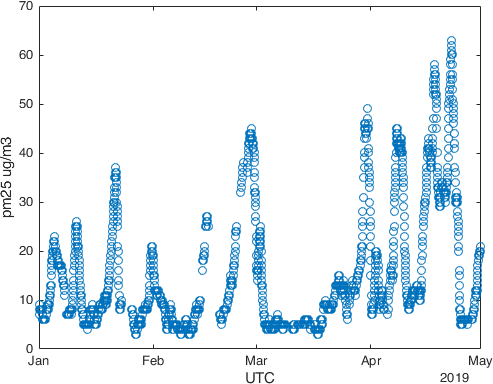
We focus on the first of the locations London Eltham, and we want to plot the
quantity of pm25 we have measured in the whole period. For doing this we need
to perform a slicing of the data. We need to find the rows that correspond to
this location, we can do this by using the command
index = strcmp(london.location,'London Eltham');
at the end of this call the variable index will be a vector having a 1 in
position i if london.location(i) is 'London Eltham', and a 0 otherwise.
With this knowledge we can now produce a plot of these values by adding to
the script
figure(1)
plot(london.utc(index),london.value(index),'o')
xlabel('UTC');
ylabel('pm25 ug/m3');
obtaining
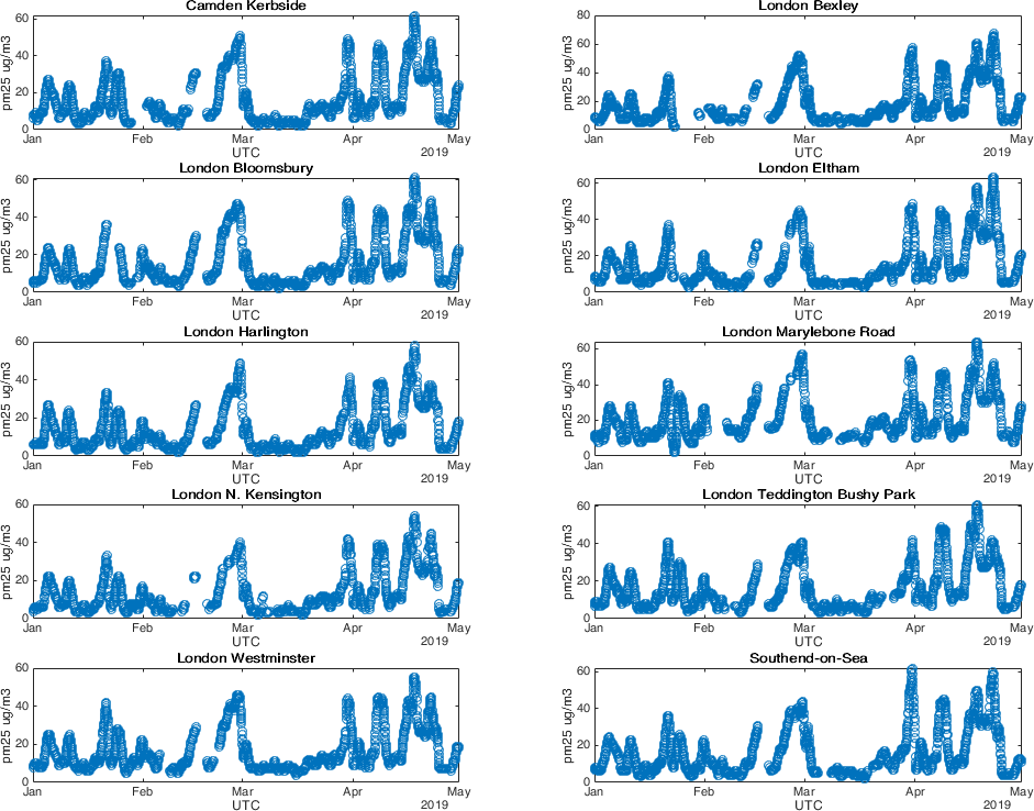
Now let us repeat the same task for all the different location. We want to
produce now a single plot with different subplots in which each of them has
one of the Locations. Since we do not want to rewrite many times the same
piece of code, we will make use of a for cycle
location = unique(london.location);

for i=1:length(location)
    index = strcmp(london.location,location{i});
    figure(2)
    subplot(5,2,i)
    plot(london.utc(index),london.value(index),'o')
    xlabel('UTC');
    ylabel('pm25 ug/m3');
    title(location{i});
end
The first line location = unique(london.location); produces, as you may guess,
the unique list of locations of our table. If we ask it on the command window,
we discover that these are
>> location

location =

  10×1 cell array

    {'Camden Kerbside'             }
    {'London Bexley'               }
    {'London Bloomsbury'           }
    {'London Eltham'               }
    {'London Harlington'           }
    {'London Marylebone Road'      }
    {'London N. Kensington'        }
    {'London Teddington Bushy Park'}
    {'London Westminster'          }
    {'Southend-on-Sea'             }
Then we loop the code for all the unique locations and repeat the same procedure
as before, with some small difference. When we look for the index vector
we now do the comparison with each and every location by looping through the
location cell array with the i index, i.e., index = strcmp(london.location,location{i});.
Then the remaining part is pretty much the same, a part from the command subplot
that tell us the number of panels in which we want to subdivide figure(2), in
this case 5 rows and 2 columns, and in which of them we are going to plot, the
\(i\)th panel at cycle i. If we run all this code, we get:
A variant of this idea could be the one of having all the plots overlapped on the same figure to do a fast comparison
Markers = {'+','o','*','x','v','d','^','s','>','<'};
for i=1:length(location)
    index = strcmp(london.location,location{i});
    figure(3)
    hold on
    plot(london.utc(index),london.value(index),Markers{i},'DisplayName',location{i})
    hold off
end
xlabel('UTC');
ylabel('pm25 ug/m3');
legend('Location','eastoutside');
from which we obtain
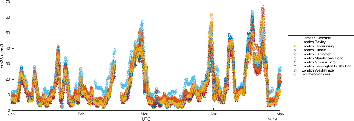
We have introduced here several new keywords,
hold onretains plots in the current axes so that new plots added to the axes do not delete existing plots.hold offsets the hold state to off so that new plots added to the axes clear existing plots and reset all axes properties.legendcreates a legend with descriptive labels for each plotted data series. For the labels, the legend uses the text from theDisplayNameproperties of the data series.
This visual comparison we have constructed is, however, rather inconclusive. Let us try producing a box plot for the different locations. This can be done with:
figure(4)
boxplot(london.value,london.location);
ylabel('pm25 ug/m3');
xtickangle(30)
that produces
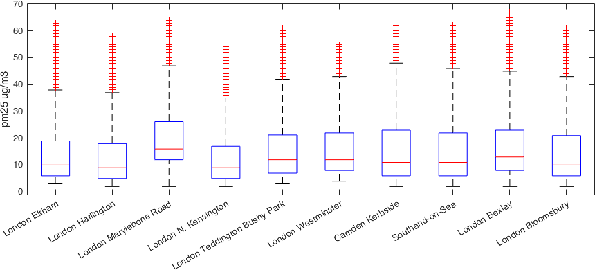
The commands we have used here are
boxplot(x,g)creates a box plot using one or more grouping variables contained ing.boxplotproduces a separate box for each set ofxvalues that share the samegvalue or values.xtickanglerotates the x-axis tick labels for the current axes to the specified angle in degrees, where 0 is horizontal. Specify a positive value for counterclockwise rotation or a negative value for clockwise rotation.
From this figure we discover that living in Marylebone Road is worse on average for the quantity of pm25.
Danger
The following part depends on having the Mapping Toolbox installed.
To conclude this part, let us put some of these information on a geographical
map. First we need to collect the latitudes and longitudes of the
different locations, then we decide that the size of the marker on the map
will be given by the mean of the values of pm25 in that location:
latitude = zeros(10,1);
longitude = zeros(10,1);
average = zeros(10,1);
for i=1:10
index = strcmp(london.location,location{i});
latitude(i) = unique(london.latitude(index));
longitude(i) = unique(london.longitude(index));
average(i) = mean(london.value(index));
end
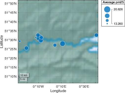
figure(5)
tab = table(latitude,longitude,average);
gb = geobubble(tab,'latitude','longitude', ...
'SizeVariable','average');
gb.SizeLegendTitle = 'Average pm25';
geobasemap colorterrain
from which we get
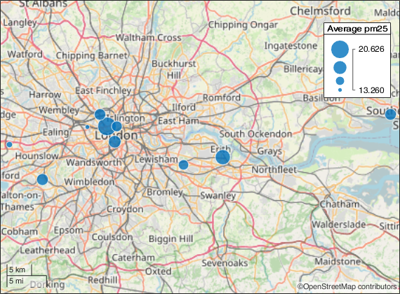
A better view using a map including the streets can be obtained by doing
figure(6)
gb = geobubble(tab,'latitude','longitude', ...
    'SizeVariable','average');
gb.SizeLegendTitle = 'Average pm25';
name = 'openstreetmap';
url = 'a.tile.openstreetmap.org';
copyright = char(uint8(169));
attribution = copyright + "OpenStreetMap contributors";
addCustomBasemap(name,url,'Attribution',attribution)
geobasemap openstreetmap
gb.MapLayout = 'maximized';
from which we obtain
Exercise 3
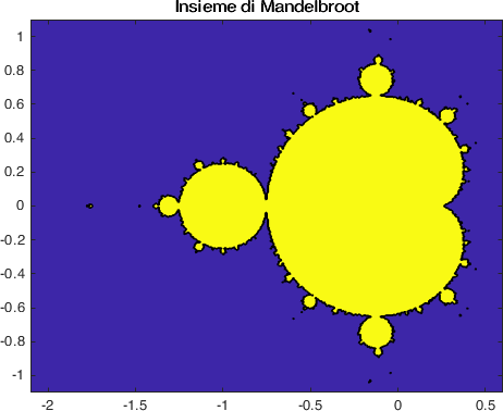
Let’s explore MATLAB’s * plot * functions again. We try to produce a print of the whole Mandelbrot fractal. This set is the set is the set of complex numbers \( c \) for which the function \( f_{c}(z) = z^{2} + c\) does not diverge when iterated starting from \( z = 0 \), that is, the set of those points \( c \) so the sequence \( f_{c} (0), f_{c} (f_{c} (0)), \ldots \) remains limited in absolute value. We can build a MATLAB script that allows us to draw an approximation of this set.
We use the
linspacefunction to construct the set of numbers \( c \) complexes on which we want to evaluate. Sincelinspaceproduces one real vector for us, we need to construct two of them – one for each direction – and transform them into a set of evaluation pairs with themeshgridfunction. A good real set to evaluate to draw the Mandelbrot set is \( [- 2.1,0.6] \times [-1.1,1.1] \).Now that we have the real evaluations, we need to transform \( c \) into complex numbers. We can do this by using the
complexfunction:C = complex (X, Y)on the pair of evaluation matrices obtained frommeshgrid.We can now implement a fixed number of iterations of the function \( f_{c} (z) = z^{2} + c \) using a
forloop.We conclude the exercise by drawing the Mandelbrot set with the function
contourf(x,y,double(abs(Z)<1e6))
title('Mandelbrot set')
which is a good chance to see what the plot function does contourf
(help contourf).
Tip
There are many others plotting functions, but we will focus on them in the following topics, while we solve problems for which they will be useful.
Writing data to screen and to file
MATLAB provides a fairly transparent porting of C’s screen printing functions (on data streams). That is, the fprintf function. For screen printing the prototype of this function is
fprintf(FORMAT, A, ...)
where FORMAT is a string that contains information about the format to be
printed and A is an array that contains the data to be printed according to
the FORMAT format. In general this is a string that can contain text accompanied
by escape characters that tell you how to format the data contained in the
A variable.
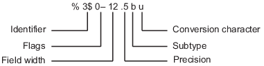
As described in the image, the escape for a formatting operator begins with
the percent sign, %, and ends with a conversion character (Table 6).
The conversion character is required. Optionally, you can specify an identifier,
flags, field width, precision, and a subtype operator between the % and the
conversion.
Carattere |
Conversione |
|---|---|
|
Intero base 10 |
|
Floating point fixed precision |
|
Floating point scientific notation |
|
Single character |
|
String |
An example:
fprintf("%f \n",pi);
fprintf("%e \n",5*10^20);
fprintf("%1.2f \n",pi);
fprintf("%1.2e \n",5*10^20);
fprintf("%c \n",'a')
fprintf("%s \n",'Ciao, mondo!')
In the example we have repeatedly used the \n characters which symbolize a
newline character. Other useful characters of this type are in
Table 7.
Result |
String |
|---|---|
Single quotation mark |
|
Percent symbol |
|
Backslash |
|
Backspace |
|
Tab horizontal |
|
Tab vertical |
|
More information can be obtained by writing help fprintf in the
command line.