Fitting data to models
Contents
Fitting data to models#
Parametric fitting involves finding coefficients (parameters) for one or more models that you want to fit to some experimental data.
In general we assume data to be statistical in nature, this means that we can assume it to be divided into two components:
the other fundamental part is that we are assuming the deterministic component to be given by a model for which the random component is described as an error associated with the data:
The model is a function of the independent data (predictor) and one or more coefficients, that are the quantities we want to compute. The error represents random variations in the data. For doing a mathematical analysis one usually assumes that they follow a specific probability distribution - in most of the case Gaussian. The source of the error can be varied, but it is always present, errors are bound to happen when you are dealing with measured data.
Least square approach#
To write down formally the idea we have discussed we can express a general nonlinear regression model as
where \(f\) is the model we want to fit, \(x_n\) is a vector of the associated variable, \(Y_n\) are the attained measurements, \(\theta\) is a vector of parameters defining the model, and \(Z_n\) is the error term.
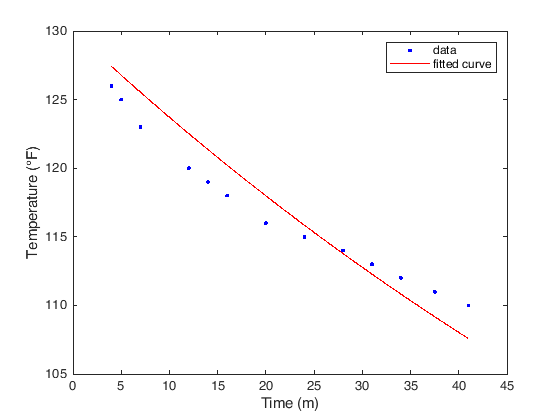
To be more practical and less formal, let us start with the tale of a certain Count Rumford of Bavaria (see [BW88]). He was one of the early experimenters on the physics of heat. In 1798 he performed the following experiment, he heated a cannon barrel to a temperature of \(130^\circ\,{\rm F}\) and then let it cool to the room temperature of \(60^\circ\,{\rm F}\) while taking measure of temperature at different time intervals:
data = [ 4 126 % Time (min) and Temperature (°F)
  5 125
  7 123
  12 120
  14 119
  16 118
  20 116
  24 115
  28 114
  31 113
  34 112
  37.5 111
  41 110
]
To interpret these data we can use Newton’s law of cooling, which states that
where \(T_0\) is the ambient temperature. This is one of the few differential equations we actually know how to solve, and indeed we can express
This model now depends nonlinearly on just one parameter \(\theta\) that is the one that we have to fit to our data. Mathematically this means that we want to find \(\theta\) such that
that is we want to solve a least square problem. Typically, together with the previous objective function we have also some constraints on the parameters. For example in this case we may want to impose the constraint of having \(\theta > 0\).
To solve these type of problems MATLAB offers a function called fit. Let us
look at its usage:
fo = fitoptions('Method','NonlinearLeastSquares',...
               'Lower',[0],...
               'Upper',[Inf],...
               'StartPoint',[1]);
ft = fittype('60 + 70*exp(-a*x)','options',fo);
[curve,gof] = fit(data(:,1),data(:,2),ft);
First we have set up some options for the
fitfunction:
in the
'Method'field we have selected the'NonlinearLeastSquares'options. This tells MATLAB that we want to solve the problem in the mathematical formulation given above.The
'Lower'and'Upper'keywords denote the bound on the parameters in the order in which they appear in the model. In our case we have just one parameter \(\theta\) so we request that0 \leq \theta \leq \infty, that is \(\theta \geq 0\).Finally, with the keyword
'StartPoint'we tell the algorithm what is the starting point of the iterative procedure producing the solution. Having good starting points for the parameters could be crucial!.
Then we fix the model we want to fit, the variable is always denote as
xwhile the other letters appearing in the expression are interpreted as the parametersWe finally launch the fit operation with the command of the same name by passing to it the data and the model we have defined.
% Array containing the data
data = [ 4 126 % Time (min) and Temperature (°F)
  5 125
  7 123
  12 120
  14 119
  16 118
  20 116
  24 115
  28 114
  31 113
  34 112
  37.5 111
  41 110
];
fo = fitoptions('Method','NonlinearLeastSquares',...
               'Lower',[0],...
               'Upper',[Inf],...
               'StartPoint',[1]);
ft = fittype('60 + 70*exp(-a*x)','options',fo);
[curve,gof] = fit(data(:,1),data(:,2),ft);
% We plot the results
figure(1)
plot(curve,data(:,1),data(:,2))
xlabel('Time (m)');
ylabel('Temperature (°F)');

The other information we can extract from the fit are contained in the two
outputs of the fit function, namely:
disp(curve)
disp(gof)
     General model:
     curve(x) = 60 + 70*exp(-a*x)
     Coefficients (with 95% confidence bounds):
       a =    0.009416  (0.0085, 0.01033)
           sse: 44.1558
       rsquare: 0.8682
           dfe: 12
    adjrsquare: 0.8682
          rmse: 1.9182
Exercise 6 (Puromycin)
We use some data on the “velocity” of an enzymatic reaction. Specifically we have measured the number of counts per minute of radioactive product from the reaction as a function of substrate concentration in parts per million (ppm). From these counts the initial rate, or “velocity”, of the reaction was calculated (\(\text{counts}/\text{min}^2\)). The experiment was conducted once with the enzyme treated with Puromycin and once with the untreated enzyme.
The velocity is assumed to depend on the substrate concentration according to the Michaelis-Menten, i.e.,
we want to
Compute the parameters \(\theta_1\) and \(\theta_2\) in the two cases (with and without using Puromycin),
Verify the hypothesis on the fact that the ultimate velocity parameter \(\theta_1\) should be affected by the introduction of the Puromycin, but not the half-velocity parameter \(\theta_2\).
data = [ % substrate treated untreated
  0.02 76 67
  0.02 47 51
  0.06 97 84
  0.06 107 86
  0.11 123 98
  0.11 139 115
  0.22 159 131
  0.22 152 124
  0.56 191 144
  0.56 201 158
  1.10 207 160
  1.10 200 NaN
 ]
Exercise 7 (Growth of leaves)
Try to find parameters for the Richards model for the growth of leaves, i.e.,
on the following data
data = [ % Time (days) Leaf length (cm)
  0.5 1.3
  1.5 1.3
  2.5 1.9
  3.5 3.4
  4.5 5.3
  5.5 7.1
  6.5 10.6
  7.5 16.0
  8.5 16.4
  9.5 18.3
  10.5 20.9
  11.5 20.5
  12.5 21.3
  13.5 21.2
  14.5 20.9
]
Fitting data to a differential model#
Until now we have always assumed to explicitly know the model. Nevertheless, such models often come as the solution of a differential equation. As we have hinted in the last topic, an explicit solution of a differential equation is usually hard to come by.
We could be in the case of having a problem of the form
depending on a set of parameters \(\theta in \mathbb{R}^m\). Then we have observations at discrete time points \(t_1,\ldots,t_p \in [0,t_{\max}]\) in the form
for a function \(g(\cdot)\) representing some observable of the system. We can state this problem again in a least square formulation as
where \(\|g(x)-g(y)\| = \sum_{i=1}^{n} |g_i(x) - g_i(y)|^2\). Thus, by manipulating a bit the quantities we have, we can use again the same strategy we have seen before.
Let us use this procedure to estimate the parameters of a SIR model. Let us proceed step-by-step
first of all we need the dynamic of the system, since we will work with uncertain data, we will run this time all three differential equations
% We order the variables as y(t) = [S(t),I(t)]
% lambda = theta(1) gamma = theta(2)
sirModel = @(t,y,theta) [-theta(1)*y(1)*y(2); ...
    theta(1)*y(1)*y(2)-theta(2)*y(2);...
    theta(2)*y(2)];
then we use the function we have seen in the last topic for integrating differential equations, this will be our workhorse, here we are using the computational resources
sirSOL = @(theta,IC,t) deval(ode45( @(t,y) sirModel(t,y,theta),t,IC),t);
now we generate our noisy data, that will represent the measurements taken on the field
% we fix the random number generator so that we generate always the same random numbers:
rng(10);
numpts=20;
tdata = [0, sort(20*rand (1,numpts))];
width = 0.1;
ndataSIR = 20*[0, normrnd(0,width,[1,numpts]);
    0, normrnd(0,width,[1,numpts]);
    0, normrnd(0,width,[1,numpts])];

lambda = 0.01;
gamma = 0.1;
S0 = 50;
I0 = 1;
R0 = 0;
theta = [lambda; gamma];
IC = [S0; I0; R0];
SIRData = sirSOL(theta,IC,tdata) + ndataSIR;
now the matrix
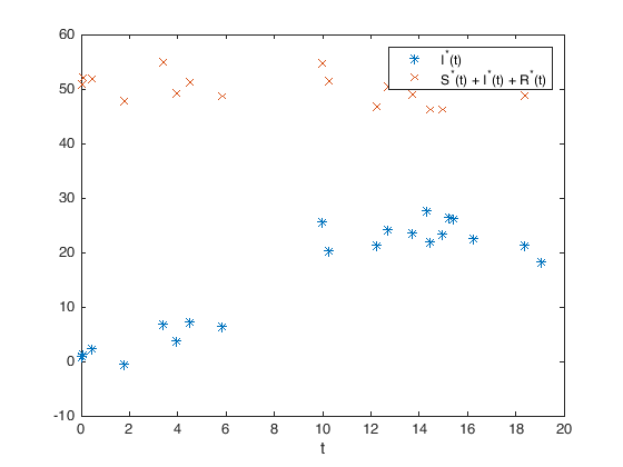
SIRDatacontains the noisy data of our system with given parameters (that are indeed the parameters that we will try to guess back). To march the optimization procedure we will focus only on the data for for \(I(t)\) and \(N(t)\)
SIRDatared = [0 1 0; 1 1 1]*SIRData;

% Let us look at the data we have obtained
figure(1)
plot(tdata,SIRDatared(1,:),'*',tdata,SIRDatared(2,:),'x')
xlabel('t')
legend('I^*(t)','S^*(t) + I^*(t) + R^*(t)')

We can now build the objective function we wish to optimize
SIRthetaSol = @(theta,t) [0 1 0;1 1 1]*sirSOL([theta(1) theta(2)],IC,t);
objective = @(theta) sum(sum( (SIRthetaSol(theta,tdata) - SIRDatared).^2 ));
that we optimize by means of the
fminconfunction. Moreover, we tell to it to print some information on the procedure, and we request that the parameters \(\lambda\) and \(\gamma\) to be in between \([0,0]\) and \([1,4]\) respectively.
options = optimset('Display','iter');
[SIRtheta, fval, exitflag] = ...
    fmincon(objective,[0.1 4],[],[],[],[],[0 0],[1 4],[],options);
Your initial point x0 is not between bounds lb and ub; FMINCON
shifted x0 to strictly satisfy the bounds.
First-order Norm of
Iter F-count f(x) Feasibility optimality step
0 3 7.527718e+03 0.000e+00 3.951e+01
1 6 7.516116e+03 0.000e+00 1.819e+03 9.864e-01
2 9 7.516075e+03 0.000e+00 6.074e+01 8.219e-04
3 12 7.515294e+03 0.000e+00 1.149e+02 1.059e-02
4 15 7.508059e+03 0.000e+00 5.941e+02 2.065e-02
5 25 7.506838e+03 0.000e+00 1.392e+01 2.104e-02
6 28 7.503699e+03 0.000e+00 4.009e+02 9.717e-03
7 31 7.502020e+03 0.000e+00 4.160e+02 1.542e-01
8 34 6.257635e+03 0.000e+00 2.477e+05 3.827e+00
9 40 5.486048e+03 0.000e+00 5.992e+04 4.682e-01
10 50 5.364982e+03 0.000e+00 9.336e+04 1.793e-02
11 53 2.821310e+03 0.000e+00 1.527e+06 4.628e-01
12 58 1.174280e+03 0.000e+00 1.647e+04 1.735e-03
13 61 1.089969e+03 0.000e+00 3.271e+05 1.275e-02
14 64 3.673265e+02 0.000e+00 7.934e+03 6.099e-02
15 75 2.999335e+02 0.000e+00 4.166e+03 2.358e-02
16 78 2.935125e+02 0.000e+00 1.041e+04 5.328e-03
17 81 2.934616e+02 0.000e+00 9.851e+03 5.052e-05
18 84 2.932380e+02 0.000e+00 7.123e+03 2.771e-05
19 87 2.929818e+02 0.000e+00 2.525e+02 1.504e-04
20 90 2.929815e+02 0.000e+00 6.330e+00 1.030e-05
21 93 2.929815e+02 0.000e+00 1.325e-02 3.758e-07
Local minimum possible. Constraints satisfied.

fmincon stopped because the size of the current step is less than
the value of the step size tolerance and constraints are
satisfied to within the value of the constraint tolerance.
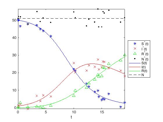
In the final step we can print the results we have obtained to screen:
tsol = linspace(0,max(tdata),400);
SIRSOL = sirSOL(SIRtheta,IC,tsol);

figure(1)
plot(tdata,SIRData(1,:),'b*',...
    tdata,SIRData(2,:),'rx',...
    tdata,SIRData(3,:),'g^',...
    tdata,sum(SIRData),'k.',...
    tsol,SIRSOL(1,:),'b-',tsol,SIRSOL(2,:),'r-',tsol,SIRSOL(3,:),'g-',...
    tsol,sum(SIRSOL),'k--');
xlabel('t')
legend({'S^*(t)','I^*(t)','R^*(t)','N^*(t)',...
    'S(t)','I(t)','R(t)','N'},'Location','eastoutside')
axis tight

Bibliography#
- BW88
Douglas M. Bates and Donald G. Watts. Nonlinear regression analysis and its applications. Wiley Series in Probability and Mathematical Statistics: Applied Probability and Statistics. John Wiley & Sons, Inc., New York, 1988. ISBN 0-471-81643-4. URL: https://doi.org/10.1002/9780470316757, doi:10.1002/9780470316757.

